How Memory and Interconnects Shape AI Infrastructure

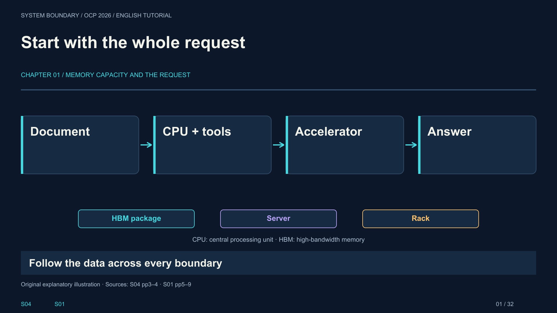
01 · Start with the whole request

Imagine an AI assistant reviewing a long technical document, checking a database, and answering a follow-up question. The accelerator may be extremely fast. Yet the user still waits. The delay might come from loading context, moving cached data, fetching a tool result, or coordinating several machines. More arithmetic alone does not remove those delays.

The central lesson from these OCP talks is that AI infrastructure is becoming a problem of placing work and data across many physical boundaries. Inside a memory stack. Between chiplets. Across a server. Across a rack. And eventually across optical links.

We will follow that path from the inside out. First, we will understand why inference creates a memory-capacity problem. Then we will examine expansion, pooling, and computation near memory. After that, we will connect those choices to chiplet interfaces, optical packaging, Ethernet fabrics, and validation. By the end, the goal is to ask sharper questions about a system proposal, even when it combines technologies from several different disciplines.

02 · The three memory questions

Start with three separate questions. How much data fits? How quickly can we move it? And how long does an individual access take? These are capacity, bandwidth, and latency. They interact, but they are not interchangeable.

High-bandwidth memory, or HBM, places stacked memory close to an accelerator. It provides a very wide data path. That makes it valuable for repeatedly feeding computation. But capacity is finite, and adding capacity inside the package has costs in area, power, packaging complexity, and cooling.

A larger memory tier outside the accelerator may solve a capacity problem while introducing a transfer problem. Conversely, a faster link cannot help if the reusable data has already been evicted because the tier was too small.

Think of a factory. Capacity is warehouse space. Bandwidth is the loading dock's sustained handling rate. Latency is the time before a particular part arrives. A good factory needs all three matched to the production schedule. An inference system needs them matched to the actual request pattern.

03 · What the KV cache remembers

The key-value cache, usually called the K V cache, stores intermediate attention information from previously processed tokens. In an autoregressive language model, retaining this information avoids repeating part of the work as the model generates additional tokens.

There are two useful stages to distinguish. Prefill processes the input context. Decode generates the answer incrementally. Time to first token measures how long the user waits before the answer starts. Inter-token timing describes how the answer continues after that.

Longer contexts create larger caches. More simultaneous sessions multiply the amount of live state. Reusing a shared document or system prompt can save computation, provided the relevant cache is still available when the next request needs it.

Micron's talk makes a particularly useful distinction: shared prefixes and active session histories are different populations. A reusable document prefix may tolerate placement in a larger, slower tier. An active session's frequently accessed state can be much more bandwidth-sensitive. Calling both simply “the cache” hides the placement decision we actually need to make.

04 · The capacity cliff

Here is an illustrative example. Suppose each active session needs two gigabytes of cached state, and a tier has one hundred gigabytes available for that state. Fifty sessions fit. Sixty do not. Actual systems also need memory for weights, buffers, and runtime overhead, but this simplified example shows the mechanism.

As concurrency crosses the capacity boundary, the system may evict useful data, transfer more often, or recompute work. Performance can change sharply. The result is a capacity cliff rather than a smooth decline.

Micron models effective reuse as potential workload reuse constrained by available capacity. Its validation on a GH200-class system examines miss rates, capacity thresholds, and concurrency. The useful idea is broader than that platform: a workload cannot benefit from reuse that its memory hierarchy cannot retain.

Our first decision rule is therefore simple. Before buying more bandwidth, measure the working set and its growth with concurrency. Ask what fits at the target load, not just whether a single request runs quickly on an otherwise idle machine.

05 · Offload is a placement decision

Offloading means placing some data outside the accelerator's local memory. The destination might be host DRAM, an expansion device, another server, or storage. Each destination offers a different balance of capacity, bandwidth, latency, and cost.

The question is not whether offloading is universally good. The question is which data to place where, and when. A frequently reused prefix may be worth retaining in a capacity tier. Active decode state may need to stay close to compute. Cold state may be cheaper to retain elsewhere, or cheaper to recompute than to retrieve.

This last comparison matters. Saving a cached object is useful only if the full retrieval path beats the alternative for the request that needs it. Include lookup, scheduling, transfer, and conversion time. Also include contention with other work.

An architecture review should therefore start with a placement policy and a workload trace. A diagram showing a large box labeled “memory pool” is only the beginning. The system needs a reason to put each category of data in that box.

06 · The hidden CPU detour

A conventional path can offload accelerator data into memory attached to the host CPU. That is convenient because the software and hardware already understand host memory. But multiple accelerators can contend for the same host-side resources.

Astera Labs asks whether the accelerator can instead reach expansion memory through a peer-to-peer fabric path. In this arrangement, the data moves through a switch to memory controllers without requiring host DRAM to be its staging area.

The important word is path. Adding memory capacity and changing the route to that capacity are two separate improvements. A system can have plenty of memory yet still funnel traffic through a shared bottleneck.

This is similar to giving several production lines their own delivery routes instead of sending every shipment through one central loading dock. The central facility still manages the operation, but it does not have to carry every payload. For an AI server, that can also preserve CPU memory bandwidth for orchestration, retrieval, databases, and other useful work.

07 · What the Astera experiment teaches

Astera's evaluation uses four accelerators, a single host socket, a fabric switch, and four expansion-memory controllers. It runs a multi-turn Qwen3 workload through vLLM and an enhanced LMCache path.

The interesting result is how the comparison changes with prompt size. At equal capacity and short prompts, the presentation reports similar performance to host memory. As prompts get longer, the added capacity becomes increasingly important. In the longest illustrated case, the system combines expansion memory with host memory.

That sequence is more informative than a single headline speedup. It shows that the benefit depends on the workload and on what the baseline is allowed to hold. If one configuration has more capacity, part of its advantage may come from avoiding evictions, not merely from a superior transfer engine.

The software change is equally important. A multi-region allocator chooses among memory regions behind one interface. Hardware creates the available routes; the allocator decides which route each object actually uses. A usable product needs both, along with observability when allocation or transfer behavior changes under load.

08 · Draw the traffic before comparing products

Before comparing two memory systems, draw the data path in both directions. Who initiates the transfer? Where does the payload travel? Which switch, root complex, memory channel, and software layer participate? Are reads and writes symmetric?

Then label the units. Capacity is usually quoted in gigabytes or terabytes. Link speed may be quoted in gigabits per second. Application throughput may be input tokens per second, output tokens per second, or requests per second. Those numbers answer different questions.

A PCI Express peer-to-peer transfer also does not automatically mean the accelerator is using CXL memory semantics. A system can use CXL in one part of its architecture while carrying accelerator-facing traffic through PCIe DMA. Marvell's smart-memory presentation explicitly illustrates this separation.

For a management team, the practical benefit of this diagram is accountability. It identifies which supplier owns the controller, which software component owns placement, and which shared resource can saturate. Without that map, a benchmark disagreement easily becomes an argument between components that were never tested at the same boundary.

09 · Expansion pooling and sharing are different

Memory expansion gives a system more capacity. Pooling allows capacity to be assigned among consumers. Sharing allows multiple consumers to access common data under defined rules. These capabilities are related, but one does not automatically imply the others.

For example, allocating a region to one server from a pool does not necessarily mean another server can simultaneously use it as coherent shared memory. The access model, ownership, synchronization, isolation, and failure behavior must all be specified.

The Samsung and XCENA session publicly frames its subject around CXL memory for agentic AI, including pooling, sharing, and processing near memory. At the conceptual level, the motivation is straightforward. Agent workloads can have changing working sets and uneven resource needs. A flexible memory system could reduce the need to provision every compute node for its individual worst case.

But flexibility introduces a control problem. Something has to decide where capacity goes, how quickly assignments change, and what happens when a consumer fails. The memory controller is part of that answer. The system software and operational policy complete it.

10 · Move computation closer to the bytes

Now imagine that an expansion device can do more than store data. It can also compress a cache entry, prepare it for transfer, or perform another supported operation near the memory holding it. This is the idea behind processing near memory.

The opportunity comes from reducing movement or host work. If an operation reads a large amount of data and produces a much smaller result, executing near the data may save traffic. If it only adds another stage without reducing the expensive part of the path, the advantage may disappear.

Marvell's composable smart-memory talk connects memory expansion with embedded compute and software services. Its examples include cache-management work and compression. This changes the device's role from passive capacity into a participant in the serving pipeline.

The right evaluation question is therefore end to end: after adding the device-side processing time, does the application receive the needed data sooner, with acceptable quality and less total resource consumption? A faster offload engine is useful. A faster user-visible workflow is the outcome we ultimately want.

11 · Compression has a quality budget

Compression can make a fixed memory tier behave like a larger one. But there are two very different cases. Lossless compression preserves the original data exactly. Lossy methods trade fidelity for smaller size and potentially lower transfer cost.

For a KV cache, that trade can affect model behavior. A useful evaluation must include application quality, not only compression ratio. It must also include the time spent compressing and reconstructing the data, and the compute resources used for that work.

Marvell's presentation compares several cache-compression approaches and reports different space, latency, throughput, and quality-related outcomes. One implementation is explicitly incomplete. The lesson is to treat these as a multidimensional design space rather than rank them by the largest compression number.

A procurement or architecture review can make this concrete. Pick the application's quality threshold first. Then measure how many requests meet both the quality target and the latency target within the system's power budget. Compression that wins on bytes but loses on the application's answer quality has optimized the wrong objective.

12 · The agent is a pipeline

The Arm and FuriosaAI presentation brings the discussion back to the complete application. An agent calls tools, retrieves information, runs orchestration code, and invokes models. Many of those stages stress the CPU, networking, or memory system rather than the accelerator's arithmetic units.

This is why freeing CPU bandwidth can matter even when an accelerator benchmark barely changes. The CPU may use those resources to process more tool calls or keep more workflows moving. Conversely, underpowered orchestration can leave an efficient accelerator waiting.

The presentation also shows how a serving target changes capacity. A system that supports many users at twenty output tokens per second per user will not necessarily support the same number at forty. Performance must be tied to a service-level objective, or S L O.

Its joint Arm-host system is a validation direction, while the illustrated Furiosa serving numbers use an x86 host. Keep those boundaries intact. The transferable lesson is to measure the complete pipeline and the complete power envelope before converting a component-level efficiency claim into a rack-level business case.

13 · Why custom HBM changes the design boundary

So far, we have expanded outward from the accelerator. Now look inward at the HBM stack. The stack includes memory dies and a base die that connects the memory to the surrounding system. Moving more functionality into a customized base die can change where interface logic and control functions live.

Marvell's custom-HBM talk argues that this should be designed as a system: base-die functionality, die-to-die links, power delivery, and package thermals need to be considered together.

The attraction is understandable. Repartitioning functions may free valuable area on the compute die or allow interfaces better matched to the application. But the logic has not vanished. It has moved into a different physical and thermal environment.

This is a recurring theme throughout the tutorial. Disaggregation creates options by moving boundaries. Every moved boundary also creates an interface, an ownership question, and a new place to validate behavior. Custom HBM is one particularly dense example because memory, logic, packaging, and cooling meet within a very small footprint.

14 · Energy per bit becomes watts

Energy per bit can sound like an abstract interface metric. A quick calculation makes it tangible. One picojoule per bit, multiplied by one terabit per second, is one watt. At ten terabits per second, that same energy cost becomes ten watts. This is illustrative arithmetic, not a measurement of any particular device.

Now add several links, memory stacks, and operating modes. Small differences in energy per bit can become meaningful package power. That is why Marvell emphasizes low-power die-to-die signaling and adaptive behavior alongside bandwidth.

But an energy claim needs an operating point. Does it describe peak traffic, a typical workload, or an idle-heavy pattern? Does it include both ends of the link? What is excluded from the power boundary?

These questions are especially important for inference, where demand may be bursty. A design that saves energy between transfers can have a different advantage from one that saves energy at full utilization. Both can matter. The comparison becomes useful only when the traffic pattern resembles the intended deployment.

15 · Heat takes a physical path

The heat generated in a package must travel through physical materials and interfaces to reach the cooling system. A stack of memory dies is a different thermal structure from a single logic die. Additional layers and interfaces affect that path.

Customizing the base die can place more activity underneath the memory stack. The resulting local temperature depends on more than the package's total watts. It depends on power density, neighboring heat sources, bonding structures, interface materials, and the geometry of the cooling path.

Marvell discusses hybrid bonding and dedicated thermal paths as part of the design space. These approaches should be understood as engineering options with process and integration requirements, rather than a universal cure for every stack.

For a semiconductor operations leader, this connects architecture directly to manufacturing execution. Bond quality, assembly variation, test coverage, and thermal characterization influence whether a promising design works consistently at volume. A package-level model should therefore be linked to measured structures and realistic production variation, not treated as a late-stage illustration after the silicon partition has been frozen.

16 · The co-design review

A useful custom-memory review brings several teams into the same conversation early. The compute architect understands the workload. The memory supplier understands the stack. The interface team understands signal integrity and transfer energy. Packaging and manufacturing teams understand assembly constraints and yield. Thermal engineers understand how heat escapes.

Each team needs a shared set of assumptions. What traffic is sustained? Where are the hotspots? Which dimensions and materials are fixed? Which performance target must survive worst-case conditions? What will be measured on test vehicles before a full product commitment?

This is not simply a request for more meetings. It is a request for a common model and clearly owned interfaces. A change that improves one die can raise the temperature of another. A narrower or more efficient interface can create room elsewhere, but only if its integration and reliability are demonstrated.

The business implication is that qualification schedule and partner coordination belong in the architecture decision. A nominal bandwidth advantage has limited value if the surrounding package cannot be manufactured, cooled, or validated within the product's intended constraints.

17 · A physical link is only one layer

When two chiplets communicate, the physical link moves electrical signals. But the system also needs agreement about what those signals mean. Is this a read request, a write, a response, a credit return, or a control message? How are errors handled? How is flow controlled?

A useful mental model separates three layers. The transaction layer describes the operation. The link layer packages and protects the exchange. The physical layer moves the bits across the actual connection.

VeriSilicon's OCE transaction-and-link-layer presentation focuses on that middle territory between a system bus and a physical interface. Its goal is to carry familiar on-chip transactions across chiplet boundaries while supporting more than one transport.

This separation can make designs more reusable. But “supports the same physical interface” is not enough to prove interoperability. Two devices also need compatible packet formats, profiles, optional features, flow-control rules, and initialization behavior. The complete conversation matters as much as the wire carrying it.

18 · What OCE TLL 2 changes

The OCE transaction and link layer version two work revisits overhead, packet formats, credit returns, and physical-layer bindings. The presentation describes support for mappings to UCIe and BoW Flexi, alongside a more generalized link-layer structure.

Why care about header size? If messages are small and frequent, headers can consume a significant share of the link. Reducing overhead can improve useful payload efficiency without increasing the raw signaling rate.

Why care about packet size? A larger link packet can spread its header cost over more payload. A smaller packet can be attractive when latency matters. These choices create a trade-off, which the specification addresses through profiles and options.

Version changes also require discipline. The presentation describes limited compatibility with the earlier generation, including specific link-layer compatibility modes. It does not promise that every version-one design can communicate with every version-two design unchanged.

The practical takeaway is to ask suppliers for an exact interoperability profile and test evidence. A standards logo tells you the family. The profile tells you which members can actually work together.

19 · Why a simpler interface still matters

BoW Flexi addresses another part of the market. Its objective is a simple, configurable chiplet link where cost, power, and implementation effort can matter more than maximum bandwidth.

The presentation describes single-data-rate signaling, a frame signal, and a minimal six-pin interface. Configuration uses the same link rather than requiring a separate sideband path. Optional fields allow the protocol to support different system needs.

This is valuable because not every chiplet is a giant compute engine. A control, analog, memory-mapped, or other modest-bandwidth function may benefit more from a small, understandable interface than from the fastest available PHY.

Think about a factory's communications. The conveyor-control signal does not need the same infrastructure as a high-resolution inspection camera. Both need dependable communication, but their cost and performance envelopes differ.

Keep BoW Flexi distinct from the higher-speed BoW S P optical example we will discuss shortly. Their rates and implementation assumptions are different. Interface complexity should earn its place through a real workload requirement, particularly across process nodes and packaging choices.

20 · Interoperability is a product outcome

We can now distinguish three things that are often collapsed into one claim. An open specification is a shared description. A compatible implementation follows the relevant rules. An interoperable product works with another implementation under the conditions customers actually use.

Moving from the first to the third requires test vectors, reference behavior, version control, and clear handling of optional features. It also requires agreement about failures: what happens during reset, a malformed transaction, a stalled peer, or a power-state change?

For a chiplet business, this affects the commercial promise of reuse. A chiplet is easier to reuse when its interface assumptions are explicit and its integration behavior is predictable. Otherwise, each new package can become a substantial custom engineering project.

This leads to a useful review question: which integration tasks disappear because of the standard, and which remain for this product pair? Ask for the answer in concrete terms. It is a better measure of ecosystem maturity than counting the number of companies that have announced support.

21 · Follow the signal into the optical engine

Optical links carry information as light, but the compute system begins and ends with electrical signals. An optical engine therefore combines photonic functions with electronics that drive, receive, and manage the signals.

Eliyan's talk makes the die-to-die interface inside this structure explicit. The electrical integrated circuit, or E I C, and the photonic integrated circuit, or P I C, must connect. In some packages, the optical engine also connects to the main compute or switch die through a die-to-die path.

This means optical architecture is partly chiplet architecture. The lane arrangement, clocking, directionality, and packaging constraints of the electrical interface need to fit the optical design.

The value of this perspective is that it prevents a black-box discussion of optics. “Replace copper with light” leaves out the conversion path, the electronic circuitry, and the connections inside the package. Those details influence energy, density, latency, manufacturability, and the choice of an appropriate chiplet interface.

22 · Fast and narrow or slow and wide

There are different ways to obtain a large aggregate optical bandwidth. One approach sends data at a very high rate through relatively few optical channels. Another distributes the traffic across more channels operating at lower individual rates.

Eliyan describes both silicon-photonics examples and slow-and-wide approaches using more optical elements. The important distinction is aggregate bandwidth versus per-channel speed. Two systems can reach a similar total while requiring very different numbers of lanes, clocks, fibers, and electrical connections.

That difference influences the die-to-die choice. Separate optical groups can have clocks with slightly different frequencies, expressed in parts per million. Grouping electrical lanes with their own clocks can accommodate those independent domains. Eliyan discusses UCIe and BoW in terms of this architectural fit rather than declaring a universal winner.

For an architecture review, start with the optical topology and work backward. How many channels are there? How are they grouped? Where does error correction terminate? Does the electrical side include retiming? Then choose an interface whose assumptions match that actual design.

23 · Bringing optics closer changes serviceability

Pluggable optics, near-packaged optics, and co-packaged optics place the optical conversion at different physical distances from the main chip. Moving it closer can reduce the difficult electrical path and create opportunities for better density or energy efficiency.

It also changes the operational boundary. A front-panel module is physically different from an optical engine integrated into a high-value package. Access, replacement, thermal coupling, and fault isolation need to be designed around that difference.

Celestica's presentation emphasizes that co-packaged optics is an enabling technology within a larger platform. It connects optics to software, management interfaces, telemetry, qualification, and service workflows.

That is a useful corrective to evaluating the technology solely through picojoules per bit. A deployment needs to know which component failed, what can be replaced, how the failure affects other resources, and how long restoration takes.

The strongest platform proposal therefore explains both the healthy path and the repair path. Efficient communication creates value during operation; clear serviceability helps preserve that value when components age, drift, or fail.

24 · Optical health must be visible

What should an operator see? Celestica highlights measurements such as temperature, optical power, external-laser performance, and error rates before and after forward error correction.

Forward error correction, or F E C, can repair certain errors. That means a link can appear healthy at the application level while its underlying error rate is getting worse. Observing only the corrected output may hide a shrinking margin.

Combining optical and packet telemetry helps answer a more useful question: is a slowdown caused by congestion, a weakening optical path, a thermal issue, or a device-level fault? The measurements must share enough timing and context to be compared.

There is also an organizational requirement. Platform teams, network operators, and hardware teams need clear ownership of each alarm and action. A rich telemetry stream is of limited use if no one knows which signal should trigger investigation.

This is where open interfaces and consistent fault definitions can pay off. They help operators manage a mixed-vendor platform without translating every incident into a separate supplier-specific language.

25 · Scale up and scale out

Scale-up connects accelerators that cooperate closely on a workload. Scale-out connects larger groups of systems across a broader network. The boundary can evolve with architecture, but the distinction is useful because communication patterns and latency requirements can differ.

ESUN, the Ethernet for Scale-Up Networking effort, aims to bring an open Ethernet-based approach to the scale-up domain. The presentation emphasizes fabric requirements while allowing implementation flexibility at the endpoints.

This is important commercially as well as technically. Ethernet has an established ecosystem of switches, software, tools, and operational experience. Adapting it for scale-up aims to use that foundation while addressing the demands of tightly coupled accelerator communication.

But sharing the Ethernet name does not make every deployment equivalent. Message sizes, topology, congestion behavior, recovery, and endpoint design still determine performance. The useful question is which specific features make the fabric suitable for the intended scale-up workload, and whether the entire path implements those features consistently.

26 · Small messages make overhead expensive

For large transfers, a modest header is a small fraction of the total. For short messages, the same header can consume a substantial fraction of each transmission. This is why framing efficiency matters in a scale-up fabric.

The ESUN one-point-zero presentation describes a compact header that replaces the IPv4 and UDP headers in its intended fabric context. It retains useful fabric functions such as congestion feedback, traffic-class information, flow labeling, and loop detection.

This is not simply deleting fields and hoping nothing breaks. It is choosing which functions a defined network environment needs and representing them more efficiently.

The presentation also describes later work on further header and inter-packet-gap optimization. Those items should be read as work in progress at the time of the talk, rather than silently folded into the released baseline.

For a product plan, the distinction matters. A system being qualified today needs a fixed feature set. A roadmap can explain future opportunities, but it should not substitute for the exact specification and implementation revision used in current testing.

27 · Recover errors locally

Link-level retry, or L L R, addresses a corrupted or missing exchange near the link where the problem occurs. The sender retains information long enough to replay it when the protocol calls for recovery. The receiver checks sequence and integrity and communicates the appropriate response.

Local recovery can be faster than asking a distant endpoint to reconstruct a larger exchange. But replay needs buffers, state machines, timers, and correct handling of duplicates and exceptional conditions.

It is also important to distinguish correctness from timing. A system can deliver every frame eventually and still experience a latency spike during recovery. For a tightly coordinated workload, that spike may delay other participants.

Alibaba and Keysight's test presentation makes this visible by testing normal operation and injected faults. The teaching point is to look beyond the phrase “lossless.” Ask how long recovery takes, how frequently it occurs, what traffic is affected, and whether the application still meets its tail-latency objective when the link is recovering.

28 · Credits prevent a different problem

Credit-based flow control, or C B F C, addresses receiver capacity. A sender transmits only when it has sufficient credit representing available space at the receiver. As space becomes free, credits are returned.

This differs from retry. Retry repairs an error. Credits help avoid overrunning a buffer. A robust fabric may need both, and their configuration can interact.

Distance matters because credits take time to return. A sender with too little outstanding allowance may pause even though the link could carry more traffic. Larger buffering or a larger credit window can help keep the link busy, but those resources have cost and must be sized correctly.

Traffic classes matter too. If unrelated flows share a resource without adequate isolation, one can interfere with another. The Alibaba and Keysight work tests incast, where several senders converge on one destination, as well as credit loss and recovery.

The management takeaway is concrete: qualify the fabric at the intended distance, frame-size mix, and traffic pattern. A short, quiet laboratory link does not exercise the same constraints as a busy deployed topology.

29 · A passed test has a boundary

Alibaba and Keysight report that their switch test configuration passed twenty-two LLR and CBFC cases. They also describe a separate endpoint-IP test effort with incomplete cases. These are different scopes, and keeping them separate makes the results more useful.

The framework follows a practical sequence: configure the system, inject traffic or faults, observe device telemetry, and validate the result against defined criteria. Cross-checking external measurements with device counters helps reveal errors that one view alone might miss.

For a buyer or program leader, ask what a pass actually covers. Which devices, firmware versions, cable lengths, frame sizes, and features were included? Were exceptional conditions exercised? Was the test repeated with another vendor's implementation?

A test result becomes reusable evidence when those conditions are recorded. Without them, “passed” is a label. With them, it is a foundation for qualification planning, regression testing, and deciding which risks still need to be retired before deployment.

30 · Use one workload contract

We can now connect the entire story with a workload contract. Describe the model and precision, context-length distribution, concurrency, reuse pattern, output length, and service-level objectives. Include quality requirements and the power boundary.

Then evaluate each layer against the same contract. The memory team asks whether the working set fits. The software team asks whether placement and transfer policies preserve reuse. The package team checks sustained power and temperature. The fabric team checks congestion and recovery. Operations checks visibility and restoration.

This creates a fairer comparison between architectures. It also prevents a common mistake: combining the best number from one workload with the best number from a different system and presenting the result as a coherent product.

For example, higher input-token throughput does not by itself prove more users can receive answers at a fixed output-token rate. A low component power figure does not establish low rack power. Each measure can be valuable, but it must remain attached to its actual workload and system boundary.

31 · The questions worth taking into a review

If you take a short checklist into the next infrastructure review, begin with these questions. What data is hot, reusable, or cold? What changes when concurrency doubles? Where is the first shared bottleneck? Which transfers bypass the CPU, and which still depend on it?

Then ask about integration. Which functions moved into another die or device? What thermal and manufacturing assumptions follow? Which interface profile is implemented, and with which partners has it been tested?

Finally, ask about deployment. What happens during a link error, a lost credit update, an overloaded receiver, or an optical fault? Which measurements let an operator distinguish those cases? How quickly can the service recover?

These questions connect technical choices to business outcomes. They influence usable capacity, energy consumption, qualification effort, deployment schedule, and customer experience. They also help identify where a supplier's component is genuinely differentiated and where the remaining work belongs to the system integrator or software ecosystem.

32 · The architecture follows the data

The twelve talks fit together because they examine different boundaries around the same workload. Micron explains why reuse depends on capacity. Astera changes the route to expanded memory. Samsung and XCENA frame pooling and near-memory work for agentic systems. Marvell explores smart memory and the physical design of custom HBM. Arm and FuriosaAI reconnect those choices to the complete inference pipeline.

VeriSilicon and BoW Flexi address the conversation between chiplets. Eliyan shows how those interfaces enter optical engines. Celestica extends the view to a serviceable optical platform. ESUN defines features for open scale-up fabrics. Alibaba and Keysight show why those features need systematic validation.

The unifying principle is to follow the data. Where does it live? How often is it reused? Who moves it? What does each boundary cost? And what evidence shows that the whole path works under the intended load?

Once those questions are answered, bandwidth, capacity, chiplets, optics, and software stop being separate product categories. They become coordinated choices in one system designed to deliver useful AI work reliably.